Introducing two new Excel functions: GROUPBY and PIVOTBY

Two new functions were announced last week: GROUPBY and PIVOTBY.

These provide a powerful yet simple way to perform data aggregations using a single formula thanks to Excel's dynamic array calculation engine.

If you’ve ever used regular PivotTables, you’ll know how great and intuitive they are. However, they do have a few downsides, such as not being as versatile as formulas and their inability to instantly update, so I'm sure this alternative is bound to sound tempting.

Before you get too excited, both functions are currently only available to Microsoft 365 Insiders on the Beta Channel (at the time of writing), so you'll have to wait a while before they reach the production version. That’s one good reason to become an Insider!

GROUPBY

GROUPBY aggregates a range of values by row group.

The full syntax is:

=GROUPBY(row_fields,values,function,[field_headers],[total_depth],[sort_order],[filter_array])

It contains three compulsory arguments:

• row_fields — the column you want to group by.‍
• values — the values you want to aggregate.
• ‍function — the function you want to aggregate them with (e.g. SUM, AVERAGE, COUNT).

Let’s look at a basic example in action.

Here’s a range containing some sales data.

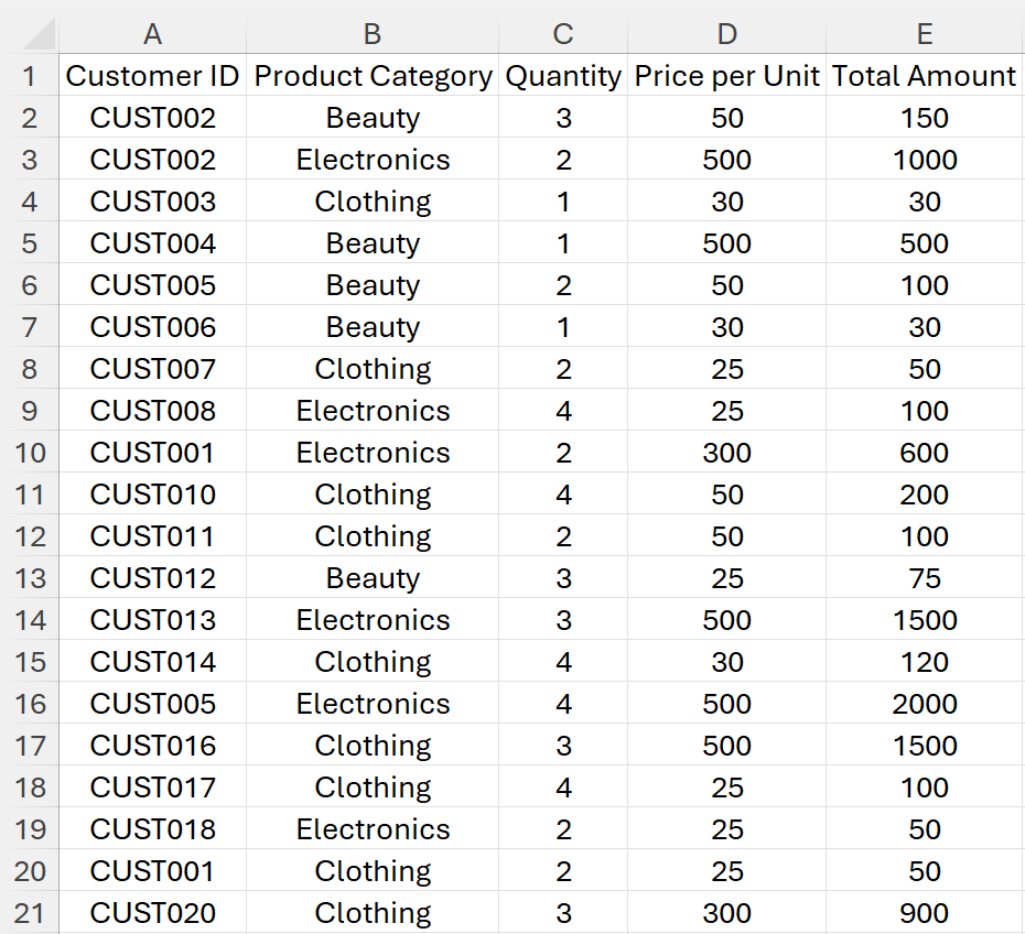
We want to find the sales for each category. Therefore, we’re interested in two columns: Product Category and Total Amount.

Inside GROUPBY, reference B1:B21 (Product Category) in the row_fields argument. Then do the same for E1:21 (Total Amount) in values. Both of these ranges include the header.

In function, specify SUM to add up the values.

The formula reads: 

=GROUPBY(B1:B21,E1:E21,SUM)

It returns the three unique values in the Product Category column and sums the Total Amount values belonging to each. The default Total row is also included.

At this point, you’ve seen the minimum required for GROUPBY to work. Let’s move on to the optional arguments.

• [field_headers] — a number that determines whether column headers should be shown and in what way.‍
• [total_depth] — a number that determines whether the row headers should contain totals.
• ‍[sort_order] — a number that indicates how the rows are sorted.
• ‍[filter_array] — a condition that determines what row_fields groups should or shouldn't be included.

Continuing with the same example, headers can be displayed by choosing 3 for [field_headers].

Notice there's a bug here, as only the first field header is showing.

However, if the reference is adjusted to include the adjacent column (D1:E21), they all appear.

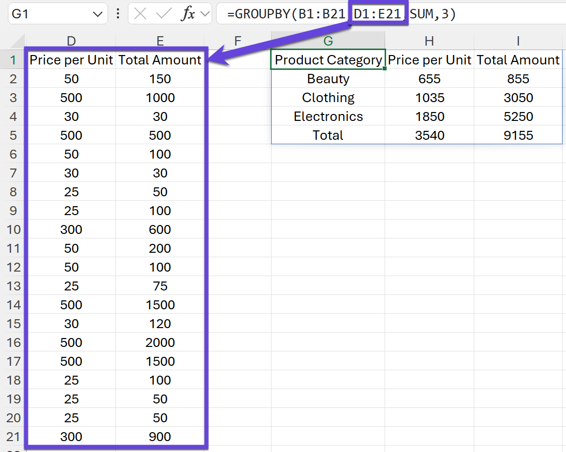
As helpful as the Total row is, there'll be times when there's a good reason to hide it. Thankfully, specifying 0 in total_depth does this, although I'll omit this for the rest of the example.

=GROUPBY(B1:B21,E1:E21,SUM,3,0)

At this stage, the totals are are in ascending order, when descending is preferable. In [sort_order], putting 2 sorts the data by the Total Amount column, which is already happening anyway. However, preceding it with a minus (-) changes the order to descending.

=GROUPBY(B1:B21,E1:E21,SUM,3,,-2)

If you want to limit what's returned, include a condition in [filter_array]. In this case, we want to return every product category except "Electronics", so reference the Product Category column (B1:B21) and use the not equal to operator (<>) followed by the string.

=GROUPBY(B1:B21,E1:E21,SUM,3,,-2,B1:B21<>"Electronics")

PIVOTBY

PIVOTBY aggregates a range of values by row and column group.

The full syntax is:

=PIVOTBY(row_fields,col_fields,values,function,[field_headers],[row_total_depth],[row_sort_order],[col_total_depth],[col_sort_order],[filter_array])

Notice the additional arguments for columns and the renamed row ones? This function is similar to GROUPBY, but being able to group by column as well gives you added flexibility.

Using the same data as last time, let's reference the Customer ID column (A1:A21) in row_fields, the Product Category column (B1:B21) in col_fields, Total Amount (E1:E21) in values, and specify SUM as the function.

=PIVOTBY(A1:A21,B1:B21,E1:E21,SUM)

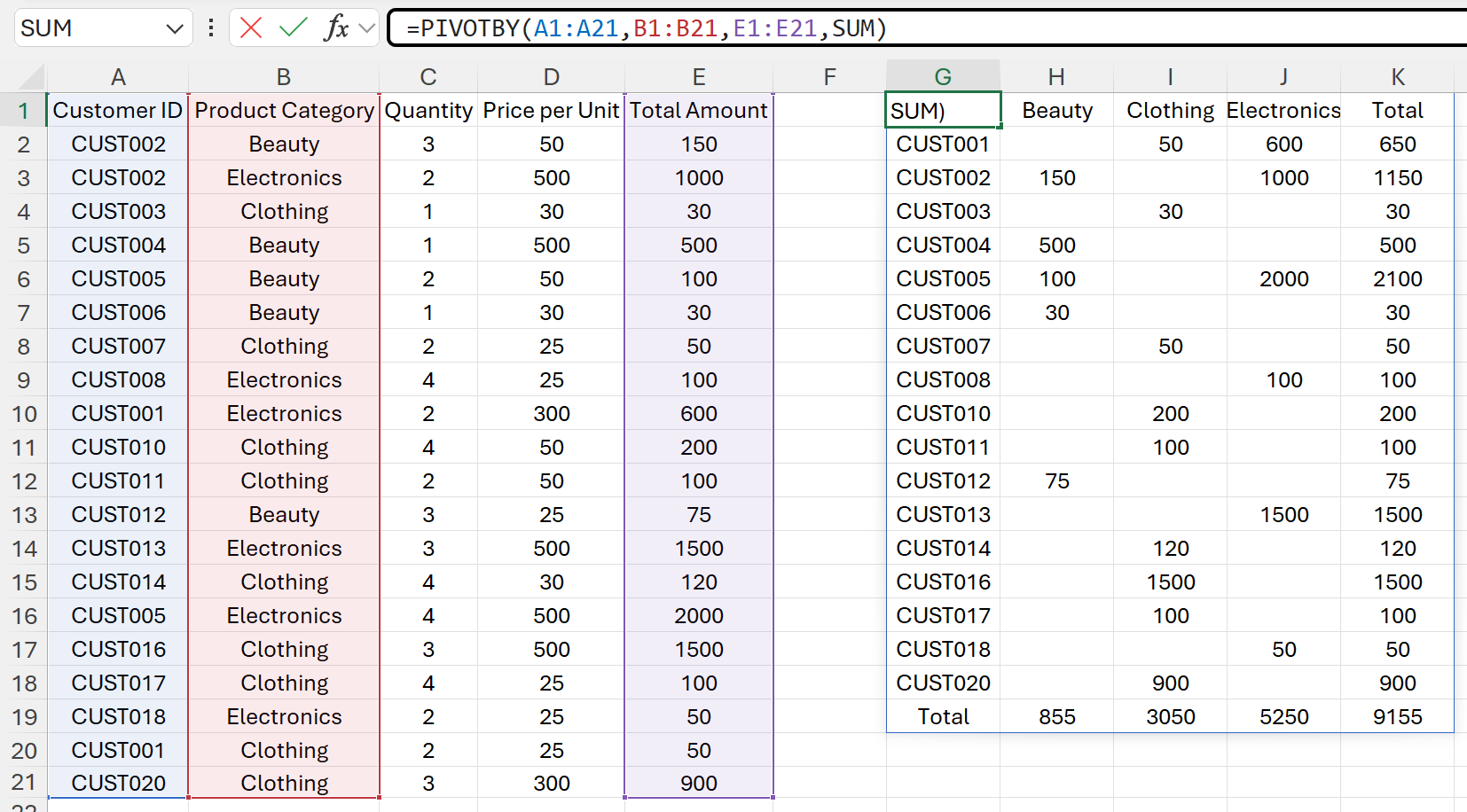
Now we have a table that shows how much customers have spent on each category.

The biggest advantage over PivotTables

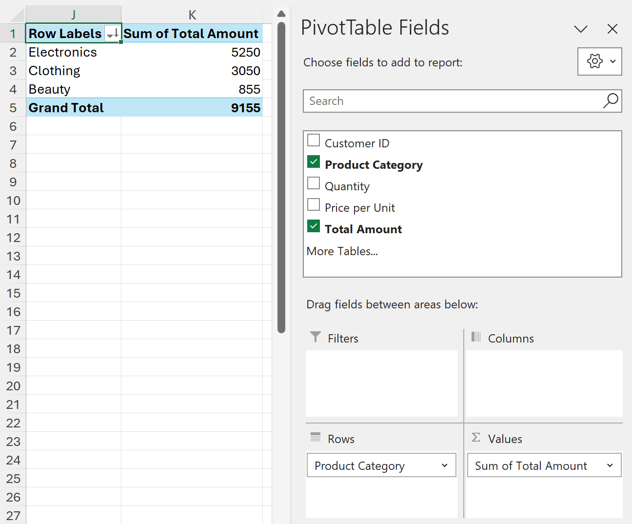
We can easily recreate the GROUPBY and PIVOTBY examples using PivotTables.

Let me quickly remind you of how to create a PivotTable…

Select anywhere in the data range and on the Insert tab, click PivotTable and then From Table/Range.

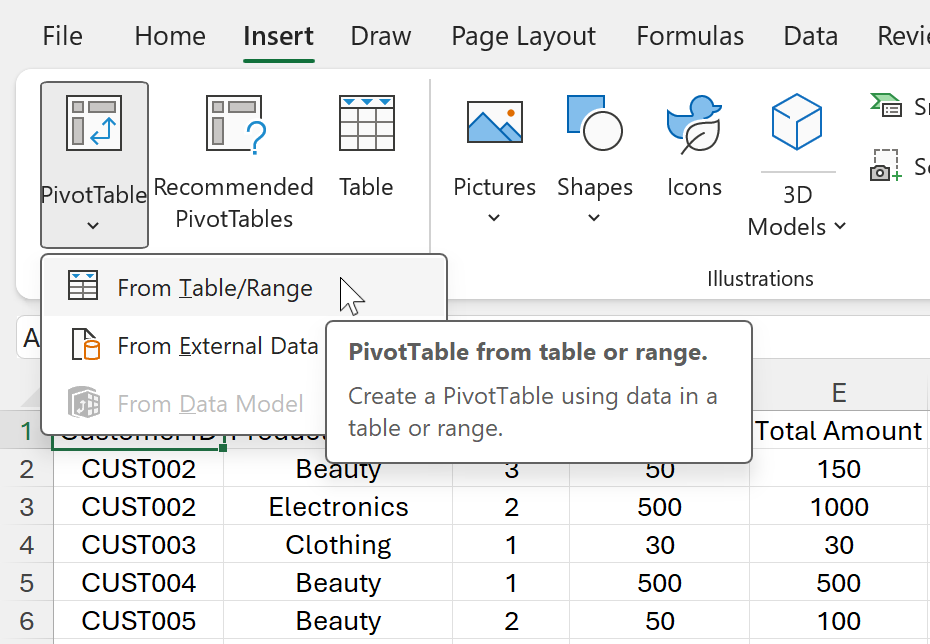
Choose a location for the PivotTable and select OK.

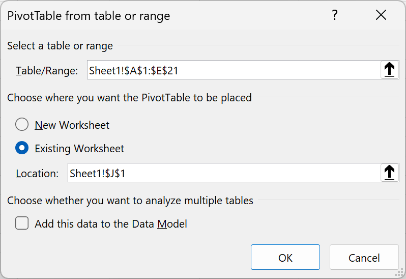
Here's GROUPBY's setup.

And here's PIVOTBY's. We'll use this one for the example below.

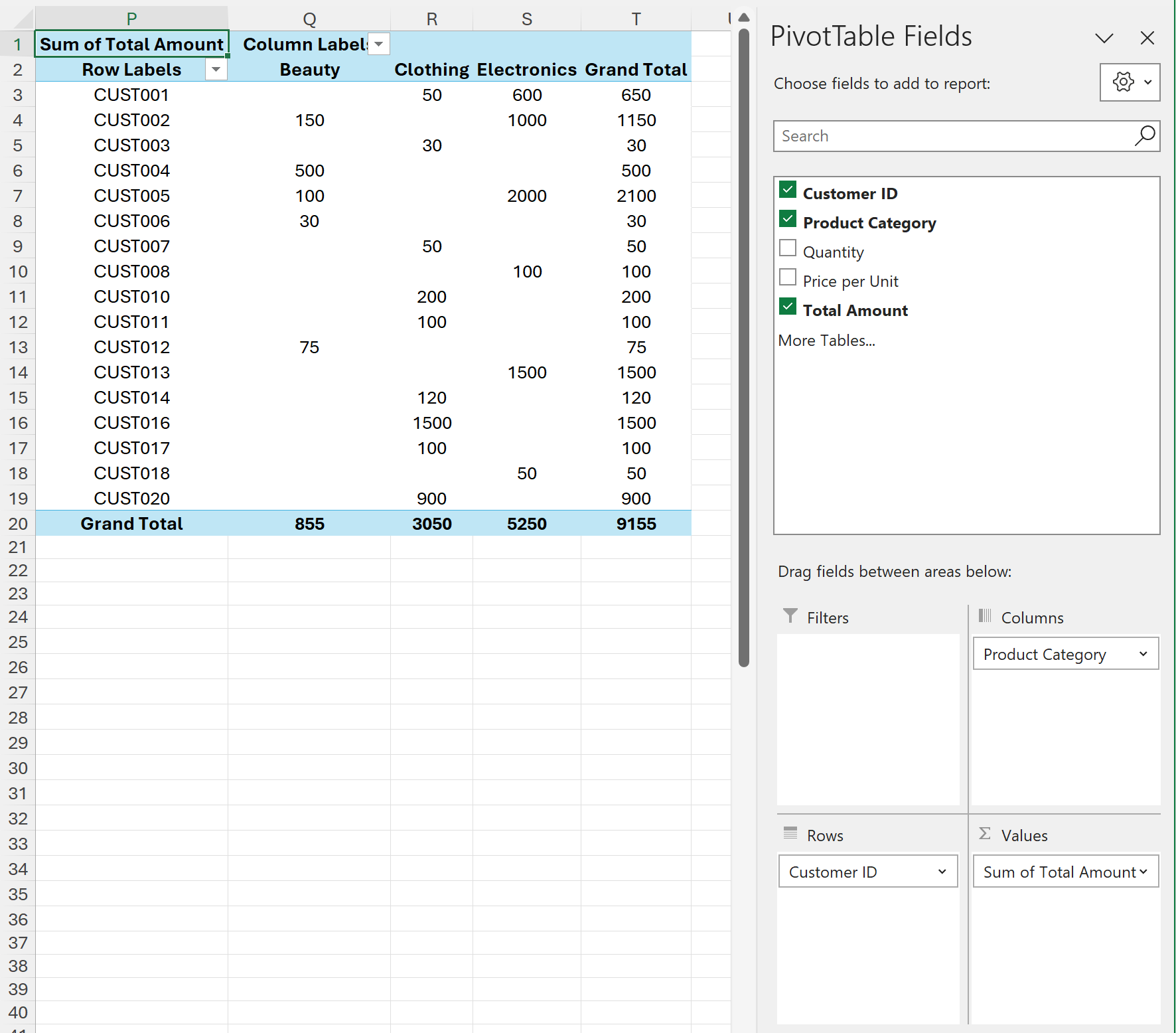
Let's change the first Customer ID entry in the source data from CUST002 to CUST001.

You might just notice a flicker in your peripheral vision. That's because the value 150 in H3 has moved to the row above in the PIVOTBY formula result.

However, cast your eyes over to the PivotTable, and you'll see it's still stuck in the previous state.

To update it, right-click anywhere on the PivotTable and select Refresh.

‍

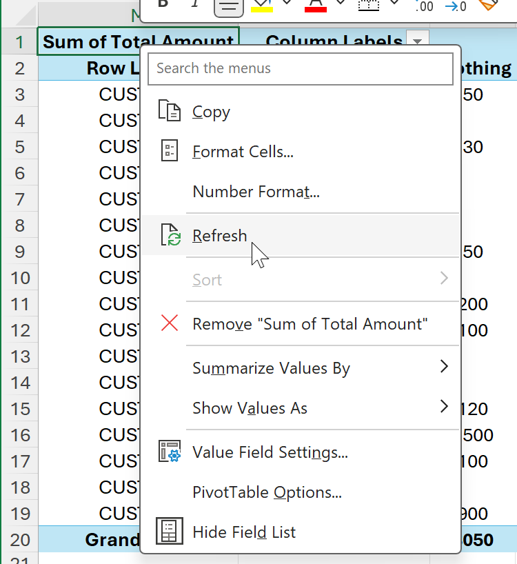
Great! It's now up-to-date.

For all the plus points about PivotTables, this is one of their fundamental flaws. Unless you want to go down the VBA route, you are stuck with this manual method.

Watch the video

Conclusion

GROUPBY and PIVOTBY are beta functions, so you might notice a few bugs, such as column headings not appearing and missing AutoComplete boxes for arguments. No doubt these issues will be ironed out, though.

Nevertheless, it provides a promising glimpse into the future.

Will you still need to use PivotTables? Well, probably if the following apply:

• You're working with a huge dataset that outsizes the worksheet grid.
• You want to display multiple aggregations, such as the sum, average, and count (this is possible but difficult to do with GROUPBY or PIVOTBY)
• You have a dusty old Excel copy instead of a Microsoft 365 one.

If you've already played around with the functions, what are your initial impressions?